This blog assumes basic knowledge of state representation and action
representation, and provides a concise comparison of multiple
reinforcement learning methods.
References include Lilian Weng’s A (Long) Peek into Reinforcement
Learning
and course PPTs from CentraleSupelec.
Policy Definition
A policy is a mapping from state to action:
Dynamic Programming (DP)
Dynamic Programming assumes full knowledge of environment dynamics
(transition probabilities and reward function).
Two steps: - Policy evaluation: Estimate
Generate
Generalized Policy Iteration (GPI) algorithm:
For step in [K1, K2, K3...]
    Policy Evaluation:
    Stop when V_(t+1)(s) = V_(t)(s)
Policy improvement
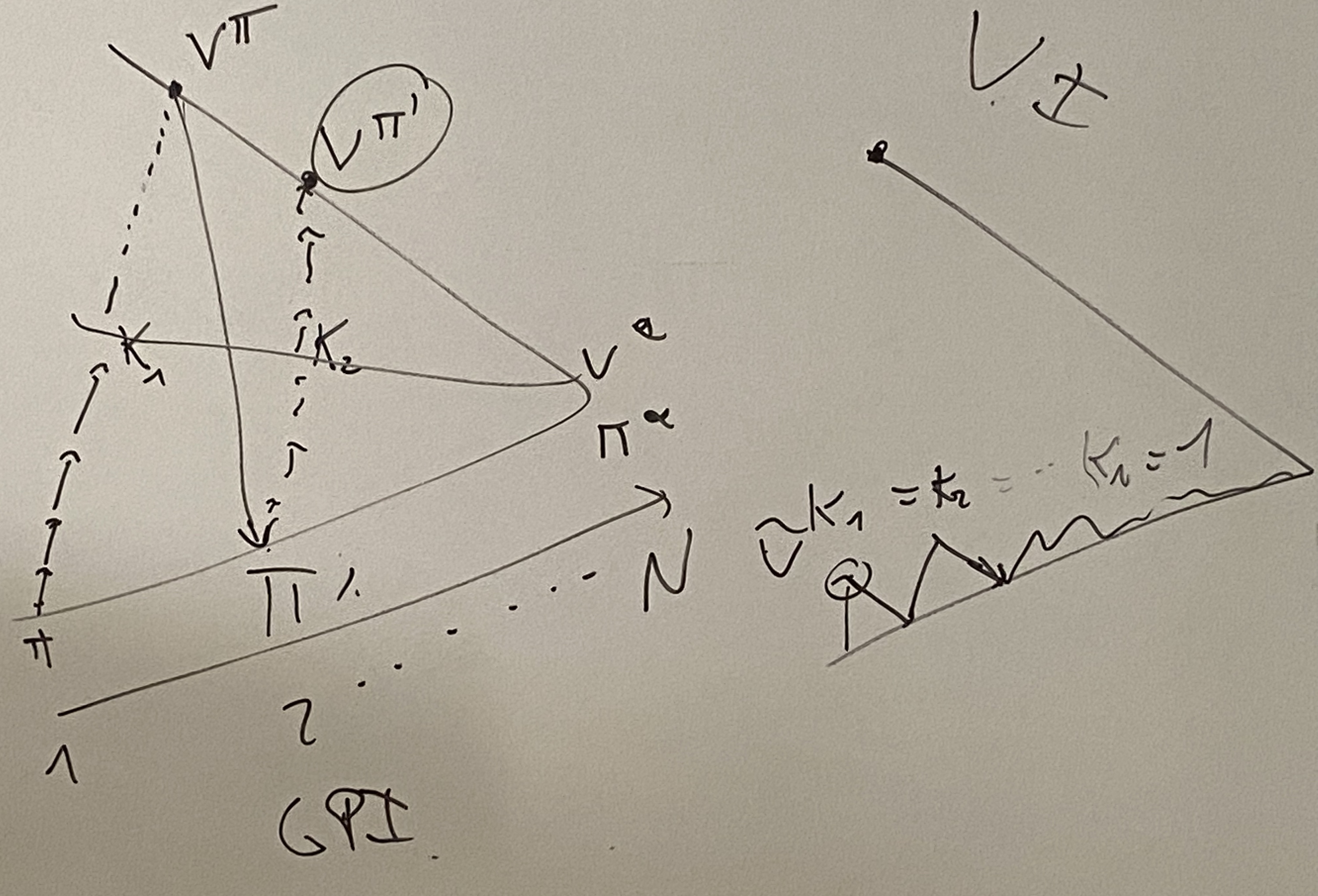
Left: policy iteration, stop after K steps or convergence.
Right: value iteration, where optimization happens at every step.
Similar to SARSA and Q-learning.
Sample Backup Methods
Traditional DP solution: full-width backups.
New methods: sample backups — using sample averages instead of full
model expectation.
Advantage: model-free, breaks curse of dimensionality.
Monte-Carlo
Using sampled trajectories:
Temporal-Difference Learning
Estimate with
Comparison of Three Methods
Method Bootstrap Bias Variance Backup
DP no 0 0 full, shallow
MC no 0 high sample-based, deep
TD yes yes low sample-based, shallow
On/Off-policy
SARSA and Q-learning are TD Learning extensions.
On-policy
The generated trajectories are based on the current policy (e.g., SARSA
with
Off-policy
Off-policy learning evaluates target policy
by a different behavior policy
Importance sampling is used for correction.
Importance Sampling Correction
Q-Learning: Off-policy TD Control
The evaluation policy is greedy:
Double Q-learning
Introduced to address overestimation in Q-learning.
SARSA: On-policy TD Control
SARSA uses
Deep RL
Table-based drawback: poor scalability.
Loss function:
DQN
Represents: - Value function
Off-policy, greedy action selection.
Value Function Approximation
Problems: - Correlation between samples (especially consecutive
states) - Non-stationary targets
Solutions: - Experience Replay - Fixed target network
Other options: eligibility traces, Dyna-Q planning, parallel
environments.
Deadly Triad
Combination of Experience Replay + Bootstrap + DL may diverge.
In practice, often converges (“soft divergence”).
Solution: multiple target networks.
Policy Gradients
Comparison
- Model-based RL: computing policy is expensive.
- Value-based RL: value error can amplify into large policy error.
- Policy-based RL: optimizes directly, but risk of local optima and
poor generalization.
Stochastic Policy
Unlike deterministic MDPs, partially observable problems require
stochastic policies.
Contextual Bandits
One-step policy gradient:
Policy Gradient Theorem
where
Drawback
Policy gradient variance is high.
Solution: KL-divergence regularization.
Then maximize
REINFORCE
Monte-Carlo trajectories with advantage
Actor-Critic
Updates both policy and value:
Asynchronous Advantage Actor-Critic (A3C)
Asynchronous threads, advantage function updates.
Gradients are aggregated and synchronized.
Modern Algorithms
- TRPO: Trust Region Policy Optimization
- PPO: Proximal Policy Optimization
- DDPG: Deep Deterministic Policy Gradient (continuous action spaces)
- A2C: Advantage Actor-Critic (advantage estimates)
- A3C: Asynchronous Advantage Actor-Critic (faster convergence)
- SAC: Soft Actor-Critic (off-policy, double-Q trick, entropy
regularization)
Online vs Offline RL
Aspect Offline RL Online RL
Data source Fixed historical dataset Real-time environment
interaction
Exploration None Active exploration
Use cases High-risk domains Simulation, games,
(healthcare, finance, robotics
recommendation)
Challenges Distribution shift, dataset Sample inefficiency,
quality dependency safety risks
Advantages Safe, reuses existing data Theoretically optimal,
continuous improvement
Summary: Offline RL is safer and suited for domains where exploration is
impossible. Online RL is powerful for environments where continuous
exploration is feasible.